TIF processing pipeline#
The ImagePipeline class#
Palmari provides a customizable pipeline structure for extracting localizations and tracks from PALM movies.
These steps are handled by the ImagePipeline class.
It is very easy to instanciate a default pipeline, containing only the minimal localization and tracking steps with default parameters :
from palmari import ImagePipeline

tp = ImagePipeline.default_with_name("my_pipeline")
A pipeline’s name is used when exporting the localizations ot the movies it processes (hey are placed in a folder named after the pipeline). Indeed, you might want to store localizations obtained using various pipelines applied on a same movie, in order to investigate the influence of the image processing step on your findings.
It takes just one line to run a pipeline on a movie or a batch of movies.
The ImagePipeline class uses Dask
to take advantage of multithreading when possible and limit the memory footprint of the processing.
By default, it will not re-process movies on which it has already been run.
tp.process(acq) # for a single acquisition
# or
tp.process(exp) # for all acquisitions of an experiment
Processing steps#
Each step of the pipeline is an instance of a ProcessingStep subclass.
Steps are divided in four main categories :
Optionally, a few movie pre-processors (subclasses of
MoviePreprocessor). Background removal or denoising steps fall into this category. These steps take as input a movie and output a modified movie.One detector (subclass of
Detector). This step (maximum one per pipeline) takes as input the pre-processed movie and outputs a dataframe containing detected spots.One sub-pixel localizer (subclass of
SubpixelLocalizer). This step refines the precision of the detected spots’ localizationsOptionally, one might have localization processors (subclasses of
LocsProcessor). These step modify localizations, add columns to the localizations table or discard localizations. They take as input the localizations dataframe as well as the original movie, and output a modified localizations dataframe. This is useful for drift correction, for instance.One tracker (subclass of
Tracker). This step links consecutive localizations of one same particle, by adding an n column, correspondoing to the particle’s ID, to the localizations dataframe. It takes as input the localizations dataframe.
Order |
Type of step |
Mandatory |
Multiple sub-steps ? |
Included |
|---|---|---|---|---|
1 |
Image processing |
N |
Y |
|
2 |
Detector |
Y |
N |
|
3 |
Sub-pixel localizer |
Y |
N |
|
4 |
Localizations processing |
N |
Y |
|
5 |
Tracker |
Y |
Y |
|
In the table, “Mandatory” means that a pipeline must have one such step. On the contrary, non-mandatory steps can be omitted. If a pipeline does not mention any particular class/setting to use for a mandatory step, the default class for this step will be used, with default parameters.
Use built-in steps#
Provided processing steps#
Palmari comes with a few built-in processing steps, which you can use to compose yout processing pipeline.
WindowPercentileFiltershifts pixel values by removing, for each pixel, the i-th hpercentile taken in a window of surrounding frames. If the pixel’s value is lower than the percentile, it is set to 0. This is meant to remove background fluorescence. Parameters are :window_size: the size of the considered window, in number of framespercentile: the threshold percentage.Detectordetects spots with a pixel-level precision. Two methods are available:llr: Perform a log-likelihood ratio test for the presence of spots. This is the ratio of likelihood of a Gaussian spot in the center of the subwindow, relative to the likelihood of flat background with Gaussian noise.log: Detect spots by Laplacian-of-Gaussian filtering, followed by a thresholding step.These methods, whose implementations were adapted from Quot, require three parameters:
w: the size of the window in which the center of the spot will be assumedt: the thresholding level above which a spot is detected.sigma: the diameter of the spots (in pixels)SubpixelLocalizerrefines the localization, using a maximum-likelihood approach. For details about the implementation, see here There are several parameters:method: a string, equal tols_int_gaussianorpoisson_int_gaussian, indicating the assumed distribution of noise.window_size: the size of the region, around the detected spot, on which the fit happenssigma: the sigma parameter of the fitted Gaussian PSFRadialLocalizerrefines the localization, using a faster but less precise approach based on radial symmetry. It has one parameter:window_size: the size of the square (in pixels) used to estimate the center of radial symmetry.CorrelationDriftCorrectorcorrects drift using time correlation between densities computed on time-wise binned localizations. Densities are simply estimated using 2D histograms. One drift vector is estimated per time bin, and the level of drift applied to each point is determined by interpolation. Parameters are :max_n_bins: maximum number of time bins.min_n_locs_per_bin: minimum number of localizations to form a time bin.BeadDriftCorrectorcorrects drift using a bead’s position. The bead is detected in the image (brightest spot) and its position over time is smoothed using a Gaussian filter. It only requires one parameter:sigma: the diameter of the bead (in pixels).ConservativeTrackertracks localizations using the Trackpy package. No missing localization is allowed (trajectories are cut if one point is missing). If there are two candidate localizations inside the search radius, the trajectory is cut as well. It takes one argument :max_diffusivity: estimation of the maximum diffusion coefficient, which defines the maximum distance between two successive localizations (search radius) : sqrt{4 D Delta t}DiffusionTrackerbuilds tracks from successive localizations using the an MTT (multi-target tracking) algorithm whose implementation was adapted from Quot, itself an adaptation of Sergé et. al. “Dynamic multiple-target tracing to probe spatiotemporal cartography of cell membranes” Nature Methods 5, 687-694 (2008). Linking options are weighted according to their likelihood, estimated via an underlying model of Brownian diffusion with diffusivity coefficient D. A linear assignment problem is then solved in order to find the optimal matching. There are several parameters:max_diffusivity: estimation of the maximum diffusion coefficient, which defines the maximum distance between two successive localizations (search radius) : sqrt{4 D Delta t}max_blinks: the maximum number of frame during which a particle is allowed to disappeard_bound_naive: the naive estimate of the diffusion coefficientinit_cost: the cost of starting a new trajectoryy_diff: the relative importance of the trajectory’s past (vs. the naive guess) in the estimation of its diffusion coefficient.DiffusionTrackersame as above but with a weighting of options simply based on the Euclidean distance. Its parameters are:max_diffusivity: estimation of the maximum diffusion coefficient, which defines the maximum distance between two successive localizations (search radius) : sqrt{4 D Delta t}max_blinks: the maximum number of frame during which a particle is allowed to disappearinit_cost: the cost of starting a new trajectory
Configure your pipeline#
We recommend using the from_dict() class method to instanciate your pipelines, specifying the desired classes and parameters in a Python dictionnary.
Steps must be grouped by categories using the movie_preprocessors, localizer, locs_processors and tracker keys.
If no localizer or tracker is found, the default classes with default parameters are used.
If a class has no parameters, simply use an empty dictionnary as a value : {"MyStepWithoutArgs":{}}.
tp = ImagePipeline.from_dict({
    "name":"default_with_percentile_filtering",
    "movie_preprocessors":[{"WindowPercentileFilter":{"percentile":10,"window_size":300}}]
})

tp = ImagePipeline.from_dict({
    "name":"stricter_than_default",
    "localizer":{"Detector":{"t":1.5}},
)
Export your pipeline’s configuration#
Pipelines can be exported and loaded from YAML files, so that they can easily be shared and re-used.
tp.to_yaml("myproject/mypipeline.yaml") # Export
tp = ImagePipeline.from_yaml("myproject/mypipeline.yaml") # Load
The YAML file for the tp2 pipeline is
name: stricter_than_default
localizer:
    Detector:
        t: 1.5
tracker:
    ConservativeTracker:
        max_diffusivity: 5.0
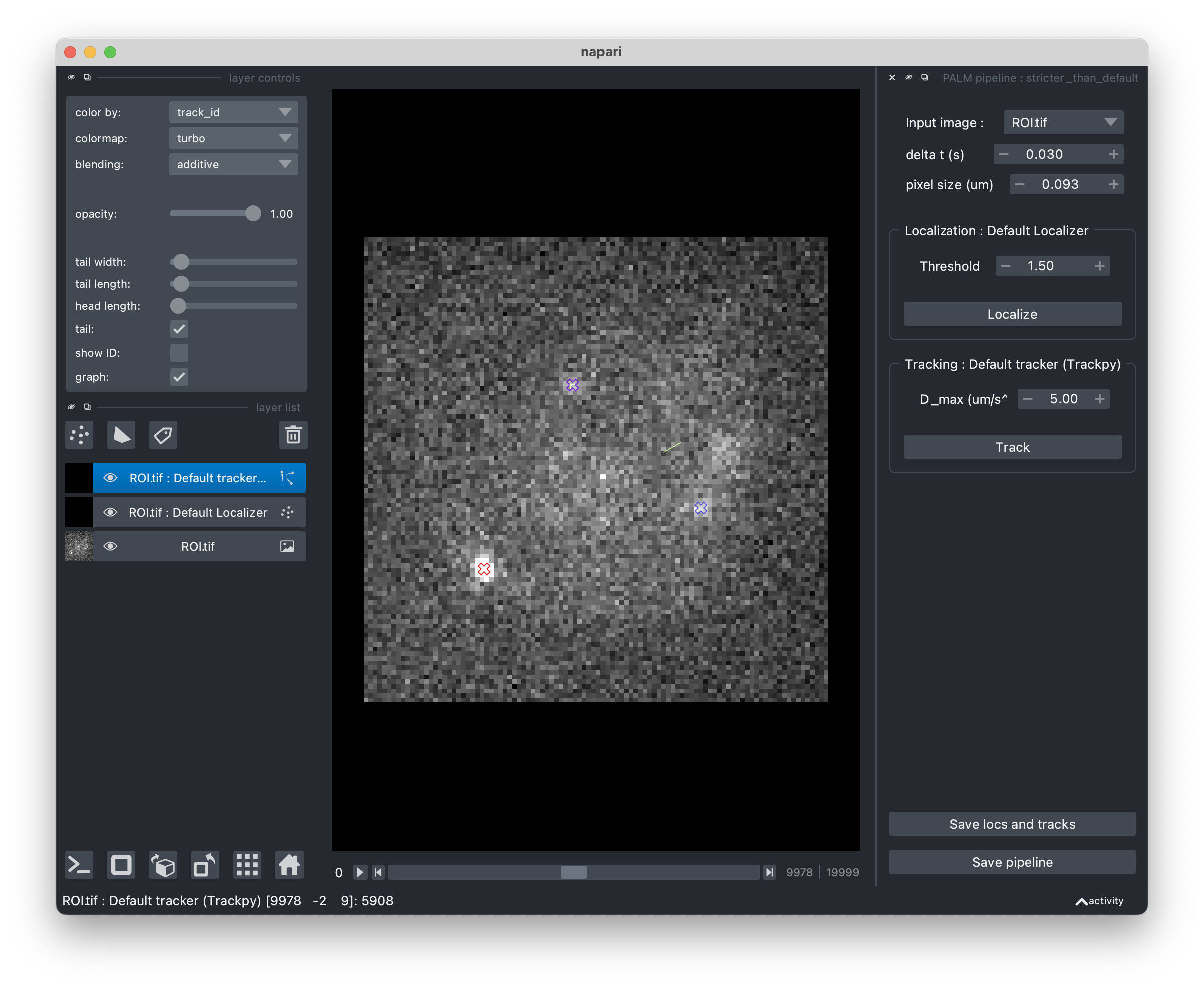
Tune your pipeline with the Napari viewer#
If you would like to adjust your pipeline’s parameters on one of your movies, you can use the ImagePipelineWidget.view_pipeline() function.
This will open a Napari viewer allowing you to see the effect of each step’s parameters on the processing of your movie.
When you’re satisfied, save the pipeline to a file by clicking the “Export pipeline” button !
You’ll then be able to load it in a script or notebook using ImagePipeline.from_yaml().
ImagePipelineWidget.view_pipeline(acq=acq)
# or
ImagePipelineWidget.view_pipeline(image_file="ROI.tif")
Make your own processing steps !#
Do you want to remove some artifact proper to your optical setup ? To use the new state-of-the-art localizer instead of the rudimentary one provided by PALM-tools (inspired from ThunderSTORM’s one) ?
Good news : the ImagePipeline class is actually quite customizable and open to add-ons !
If you want to use your own steps, subclass the corresponding abstract base class :
for a localizer, Localizer, for a movie pre-processor, MoviePreprocessor, etc…
One method must be overriden in your subclass, whose name depends on the type of step (see the code for details).
Important
Stick to the argument and output types provided in the abstract base classes for things to run smoothly.
Note that movie pre-processors’ preprocess() functions expect Dask arrays while detectors’ detect_slice() expect numpy arrays :
in this last case, Dask arrays are sliced by blocks of successive frames by the pipeline.
As an example, here is the code of the ConservativeTracker class, based on Trackpy.
The source code of BaseDetector and other built-in steps might guide you when implementing your own processing steps.
class ConservativeTracker(Tracker):

    def __init__(self, max_diffusivity: float = 5.0):
        # Attributes will automatically be detected as parameters of the step and stored/loaded.
        # Parameters must have default values
        self.max_diffusivity = max_diffusivity

    def track(self, locs: pd.DataFrame):
        # This is where the actual tracking happen.
        import trackpy as tp

        delta_t = self.estimate_delta_t(locs)  # This is a Tracker's method.
        dim = 2
        max_radius = np.sqrt(2 * dim * self.max_diffusivity * delta_t)
        logging.info("Max radius is %.2f" % max_radius)
        tracks = tp.link(locs, search_range=max_radius, link_strategy="drop")
        locs["n"] = tracks["particle"]
        return locs

    @property
    def name(self):
        # This is for printing
        return "Default tracker (Trackpy)"

    # The following dicts are used when setting the parameters through a graphic interface, using open_in_napari()
    widget_types = {
        "max_diffusivity": "FloatSpinBox",
        "delta_t": "FloatSpinBox",
    }
    # For details about widget types, see https://napari.org/magicgui/
    widget_options = {
        "delta_t": {
            "step": 0.01,
            "tooltip": "time interval between frames (in seconds)",
            "min": 0.0,
            "label": "Time delta (s)",
        },
        "max_diffusivity": {
            "step": 1.0,
            "tooltip": "Assumed maximum diffusivity (in microns per square second).\nThis is used in conjunction with the Time delta to set the maximal distance between consecutive localizations",
            "label": "D_max (um^2/s)",
            "min": 0.0,
        },
    }